Introduction to Adaptive Echo Cancellers

This paper presents a basic acoustic echo canceller based on the least mean square (LMS) algorithm. Acoustic echo cancellers are essential in many modern communication products. Do you ever hear your own voice when you talk on the telephone? This is an example of an acoustic echo. Acoustic echo is a common problem caused by audio signals bouncing off nearby objects and coupling into the microphone, which is supposed to pick up only your voice, or due to direct coupling between the speaker and the microphone (e.g., cell phones). If these effects are not eliminated, the entire communication system can be very annoying!

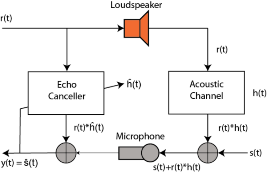
Figure 1

Here, the voice signal from the loudspeaker is acoustically coupled into the microphone of the speakerphone or handheld phone and is heard as an echo at the far end source. The echo in the system model shown in the figure can be suppressed by utilizing an echo canceller at the echo source. Assume that the sampled data impulse response of the channel is represented by the Z-transform as:

$$H(Z) = 1 + 0.5Z^{-3} + 0.1Z^{-5}$$

The echo canceller is a delay filter 50 samples long. The desired signal s(t) is first allowed to be zero and the cancellation filter is trained with white noise. The signal in Figure 1 is summarized as follows:

$$\text{speech signal}: s(t)$$

$$\text{echo}: r(t)$$

$$\text{acoustic channel}: h(t)$$

$$\text{acoustic channel output} = r(t)*h(t) \text{(convolution)}$$

$$\text{Microphone Input}: s(t) + r(t)*h(t) , \text{Desired signal plus echo through acoustic channel}$$

$$\text{Echo Canceller}: \hat{h}(t)$$

$$\text{expected signal}: y(t)$$

The goal is to match the acoustic channel through our echo canceller to invert the response of the acoustic channel and generate the desired signal (t) at the microphone input only. Here's a look at how this is accomplished in Matlab code:

clear all;clf;close all;

% acoustic channel frequency response

num = [1 0 0 0 0.5 0 .1]; den = [1 0 0 0 0 0.5 0 .1].

den = [1 0 0 0 0 0 0].

[Hc,Wc] = freqz(num,den).

% --- Build the FM sweep ---.

%fs = 2*pi.

tmax = 10000.

f1 = 0; f2 = .5.

tsweep = 0:499;

slope = (f2-f1)/1000.

F = slope.*(mod(tsweep,500));

t = 0:1:tmax.

fm = cos(2*pi*slope*t);

F = slope.*(mod(tsweep,500));

fm2 = cos(2*pi*(F). *tsweep).

fm2c = repmat(fm2,20,1).

fm2 = reshape(fm2c',1,10000 ).

figureplot([0:999],fm2(2001:3000))

%subplot(212)

%plot([-512:511]*1/(2*pi), 20*log10(abs(fft(fm2(1:500), 1024))))

grid on

% End FM sweep construction

trainlen = tmax.

%train signal

r_t = 1*rand(1,tmax).

%expected signal

s_t = 0; %Signal passes through channel

%Signal passing through channel

rt_ht = filter(num,den,r_t).

%signal passing through channel + expectation

mic_in = s_t + rt_ht;

Echo canceller for the %LMS algorithm

reg1 = zeros(1,50);

wts = (zeros(1,50));

mu = .07.

for n = 1:trainlen

   wts_sv = wts; wts_sv = wts; wts_sv = wts; wts_sv = wts

   reg1 = [r_t(n) reg1(1:49)];

   err = mic_in(n) - reg1*(wts');

   y(n) = err.

   wts = wts + mu*(reg1*(err'));

   end

% Plotting

figure

subplot(211)

plot(1:length(y), (y))

hold on

plot(1:10000, zeros(1,10000), 'color', 'r', 'linewidth', 2, 'MarkerSize', 2)

hold off

axis([ -.5 10000 -1 1.1])

grid on

title('Steady state (time response) expected signal = 0, white noise training')

subplot(212)

plot(1:length(y), 20*log10(abs(y)))

grid on

title('Log-amplitude training curve, trained with white noise')

[Hf,Wf] = freqz(wts_sv);

figure

subplot(211)

plot(Wc/pi, 20*log10(abs(Hc)))

grid on

title('Channel frequency response')

subplot(212)

plot(Wf/pi, 20*log10(abs(Hf)),'color','r')

title('Adaptive canceller frequency response, trained with white noise')

grid on

In the code, we first add the acoustic channel response to the Hc and Wc variables. We then construct an FM sweep training signal to be used in the second part of the training of the echo canceller. We then define the signals r_t, s_t, Ort_ht, and mic_in to reflect Figure 1. The focus is then on the adaptive canceler: we train it using a simple iterative least-mean-square method.

First, we define registers of depth 50. This is equivalent to an array in C or C++ (embedded applications). Then we define an empty array of weights - wts - and set $$\mu$$, an important step factor in the least-mean-square algorithm, which takes a very small step at each iteration to find the set of weights that best describes the acoustic channel and provides the smallest error for each input. the LMS algorithm is simple - we start by adding a white noise sample to the register and then calculate the error:

$$err = \text{mic_in}(n)- reg1*wts'$$

Then update the weights

$$wts = wts + \mu*(reg1*err')$$

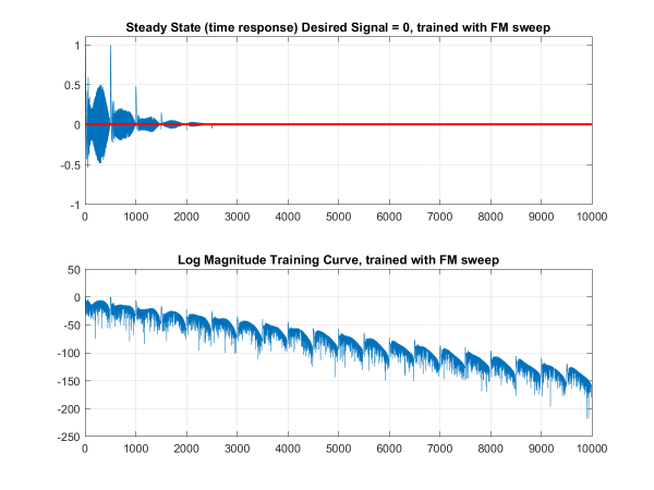
The derivation of the weight update is a lengthy explanation that will not be detailed in this article, but I will post a separate explanation later. However, the weight update simplifies to the transpose of the current weights plus $$\mu$$ multiplied by the contents of the register multiplied by the error. Letting it run until convergence, we see that after training the white noise the algorithm finds the ideal set of weights to achieve the desired signal of 0.
 
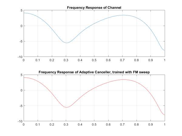
And we can see that the echo canceller response converges almost exactly to the frequency response of the acoustic channel.

If we train it without the FM signal, we can see that the convergence is slightly slower, but the error is smaller!

That's it - a few lines of code to build a pretty good echo canceller. Watch out for an upcoming article on Least Mean Methods for a more in-depth look at how the algorithm works!