Achieving Convergence for High-Q XTAL Oscillators

When using Cadence's Virtuoso Periodic Steady State (PSS) analysis for high Q crystal oscillator simulations, it is often difficult to achieve convergence and thus impossible to model phase noise, even with options specifically designed to improve convergence.

In this paper, we will discuss a method that greatly improves the probability of convergence and enables the simulation to be completed in a short period of time. This technique proved its effectiveness when the oscillator was embedded in a hierarchy of hundreds of other circuit modules.

Initial Setup

The simulation options should be set to minimize the amount of work Spectre has to do to find a solution so that accurate results are obtained when the PSS converges. Some of the default Spectre settings are overly restrictive, causing potential problems for most designs, such as “iabstol”. However, for high Q crystal oscillators, the default relative error “reltol” is not accurate enough.

The recommended starting point is:

• reltol=10e-6
• iabstol=10p
• gmin=10p

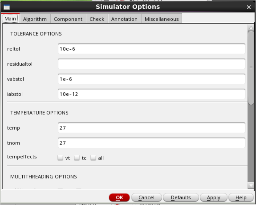
The default values for Spectre/SPICE are usually a current error tolerance of 1pA and a relative error of 0.1%. When using standard double-precision arithmetic, SPICE can only converge on variable ranges up to about 12 orders of magnitude, so 1pA is quite harsh for most circuits. For high-current circuits, it is sometimes a good idea to increase this value to 100 pA or even 1 nA. However, the default relative error of 0.1% is not enough to get reliable accuracy in phase noise.

A reasonable starting value is 10e-6, and for some circuits this needs to be increased to 1e-6. A step jump in the phase noise plot, for example, is a sign of inaccuracy.

PSS Settings

The PSS form must be set to always perform a pre-transmission run “tstab”. Numerous simulations have shown that options related to improving convergence almost always fail in oscillators that are difficult to converge. I.e. “Detect steady state” and “Calculate initial conditions” should not be enabled.

The suggested starting point is:

• number of harmonics = 50
• precision default = conservative
• Running transient = yes
• Stop Time = described below
• detect steady state = not enabled
•  Calculate initial conditions = not enabled

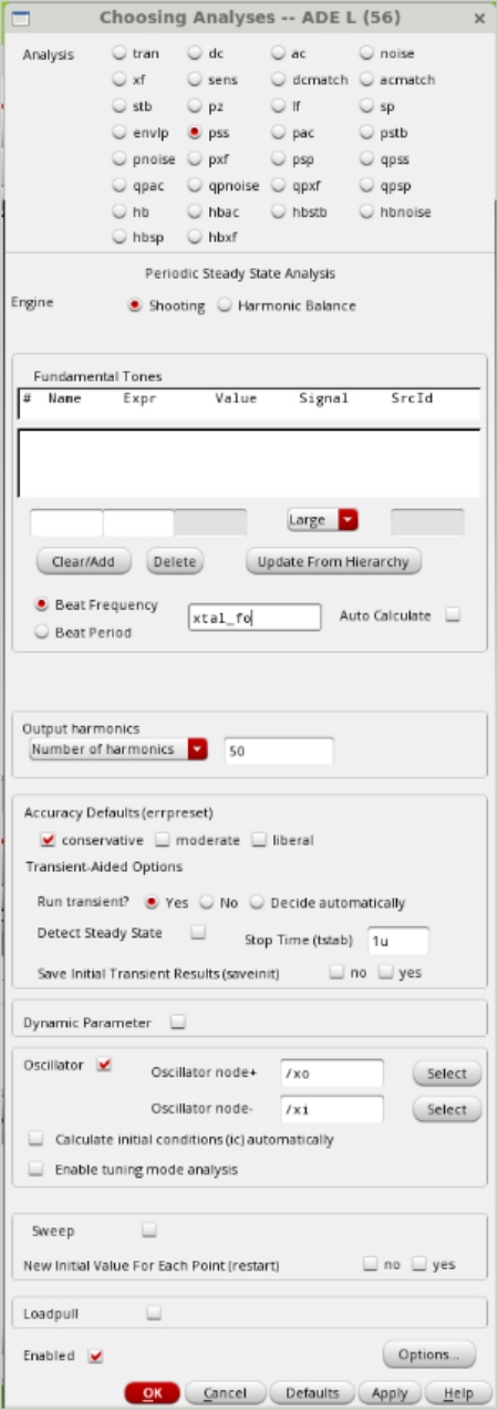
The shot method is usually the best method for any oscillator system other than a simple sine wave output. Most oscillator applications require a limiter to make the system highly nonlinear. Therefore, the default 50 harmonics is a good starting point. For particularly difficult circuits, 100 harmonics may be required. If the overall phase noise plot is not smooth, it may indicate that the plot may be incorrect. Conservative accuracy settings mean that Spectre will set the initial 10e-6 more tightly.

Note that the oscillator node is usually set to the XTAL node.

PNoise Settings

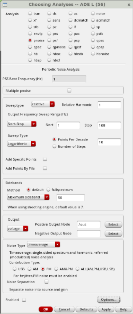
The PNoise settings are relatively standard. To ensure accuracy, the default maximum sideband is set to 50.

To minimize simulation time while still obtaining a reasonably smooth graph, a logarithmic plot of 10 points per decade is usually sufficient. Generally only phase noise is of concern, so check the appropriate box.

Output/Plotting Settings

To ensure that the oscillator is working properly, you should first run a Cadence stability analysis.

However, at the time of writing, Cadence Stability Analysis has a fundamental flaw that makes it impossible to output loop gain margins and loop phase margins via its direct plotting feature. (Despite the submission of a support work order...)

The following appears in the Cadence Spectre log:

“ WARNING (SPECTRE-16922): The phase margin and gain margin cannot be obtained because the circuit is a positive feedback system and is unstable. This is because the amplitude of the loop gain as it crosses zero degrees is greater than 1. To stabilize the circuit, make sure that the amplitude of the loop gain as it crosses zero degrees is less than 1.”

Of course, this is an oscillator after all! Anyway the output results ....

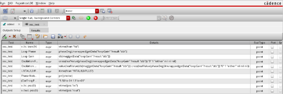
The output form should therefore be set up using a manual script as shown here:

Phase Loop

phaseDegUnwrapped(getData(“loopGain” ?result “stb”))

Gain loop

db(mag(getData(“loopGain” ?result “stb”)))

Oscillation frequency

cross(leafValue(phaseDegUnwrapped(getData(“loopGain” ?result “stb”))) “0” 1 “either” nil nil nil)

Oscillation gain

value(leafValue(db(mag(getData(“loopGain” ?result “stb” )))) cross(leafValue(phaseDegUnwrapped(getData(“loopGain” ?result “stb”))) “0” 1 ” either” nil nil nil))

Sometimes, depending on the circuit, there may be a 360 degree phase shift, so the intersection point “0” should be adjusted appropriately.

 

XTAL Model Setup

The XTAL schematic should be set up to calculate the required XTAL inductance from the XTAL c1 and XTAL frequency. Therefore, the inductance in the Inductor Setup form should be set as follows:

1/(pPar(“C1”)*((2*3.141592654*pPar(“FS”)*(2*3.141592654*pPar(“FS”) ))))

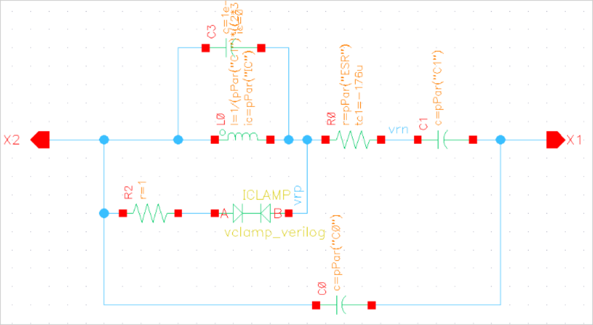
The component ICLAMP is a Verilog voltage/current limiter that helps in convergence, since XTALS with high Q can produce values of 100kV and SPICE can produce even higher voltages during convergence. It helps to avoid the “last converged node = 123.8 MV” error. However, this may not be necessary.

The code is:

`include “constants.vams”

`include “disciplines.vams”

module vclamp_verilog(A, B);

inout A.

inout A; electrical A; inout B; inout B

inout B; electrical B; inout B

inout A; electrical A; inout B; inout B; electrical B.

parameter real imax = 0.5 ;inout A; electrical A; inout B; electrical B; inout B

parameter real imax = 0.5 ; parameter real vmax = 1 ; parameter real i0 = 1E-18 ;

parameter real i0 = 1E-18.

analog begin

   I(A,B) <+imax*tanh(i0*sinh(100*tanh((40/vmax/100)*V(A,B)))); parameter real imax = 0.5 ; parameter real i0 = 1E-18; analog begin

end

The capacitor connected in parallel on the inductor is a very small value virtual capacitor, typically 1e-20 F. This is to make it convenient to set the initial voltage of the inductor to 0 V. This nodal voltage setting is part of this convergence technique.

Convergence Methods

The problem with the convergence of high Q XTALS is that Spectre has trouble converging due to the high Q values. For the same circuit, but with a lower Q, there are usually fewer problems. Therefore, the approach is to solve the low Q circuit first and use the results to help solve the high demand Q circuit.

The key principle is that a low Q XTAL reaches a steady state much faster than a high Q XTAL. i.e., if the XTAL is “de-Q'd” 100 times, then the simulation will stabilize 100 times faster.

The Q of the XTAL oscillator is determined by the C1 (series resistor) of the XTAL. However, the steady-state current of the inductor in the XTAL is independent of C1. Therefore, the low Q inductor current can be used as the initial current for a full Q XTAL.

Therefore, the principle of the method is to initialize the inductor current so that it is close to the steady state current, which is obtained by running the low Q version of the circuit first.

To set up the simulation, introduce a variable - for example, QR, which is multiplied by C1, so that QR is first set to 100 for a low Q run, and then set to 1 for a full Q run. Example:

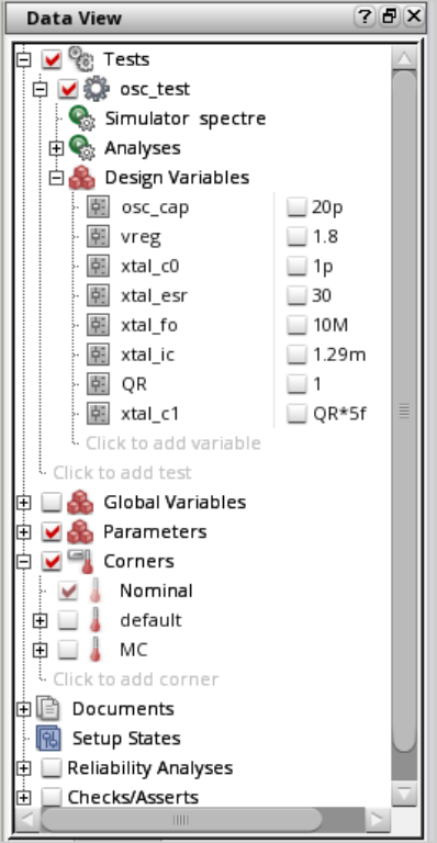
Example Schematic

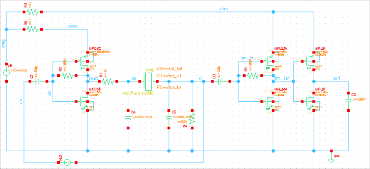
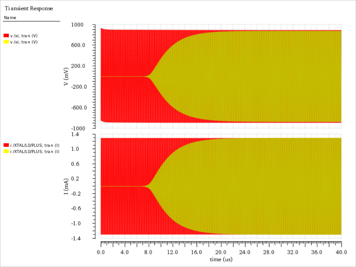
Example Waveforms

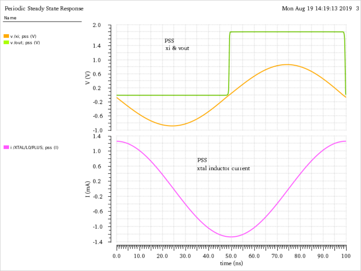
The top graph shows the X1 signal voltage for low Q and high Q operation. The bottom graph shows the inductor current for Low Q and High Q operation. As can be seen, the values determined from the Low Q configuration allow the High Q configuration to begin almost immediately. This provides better initial conditions for the PSS and thus more likely to converge. In this case, the PSS tstab time is only set to 1 us. for difficult cases, an empirical determination is required.

Transient Response

PSSR

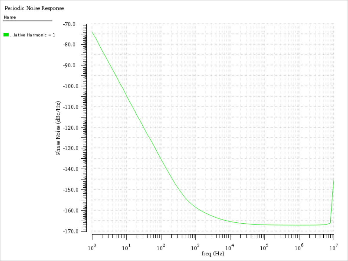
Phase noise